
Image Classification using CNN (PyTorch)
As we all know, insects are a major factor in the world's agricultural economy. Therefore, it is particularly important to prevent and control agricultural insects by using procedures such as dynamic surveys and real-time monitoring systems for insect population management. However, there are many insects in the farmland, and it takes a lot of time to be manually classified by insect experts. Since people without the knowledge of entomology cannot distinguish the types of insects, it is necessary to develop more rapid and effective methods to solve this problem.
Can a computer automatically detect pictures of insects? It turns out that, given high-quality training data, it is very straight-forward to accurately classify images of insects. In this article, I will build a machine learning model to classify images of insects using the Insect Images dataset. I will introduce step by step how to train the model, design the input and output for category classification, and finally display the accuracy results.
You can find my Github repository for this blog here.
Image Classification
The problem of image classification is this: given a set of images that are labeled with a single category, we are asked to predict these categories for a new set of images and measure the accuracy of the predictions. How will we write an algorithm that can classify images into different categories? Computer vision researchers have proposed a data-driven approach to solving this problem. Instead of trying to directly specify in the code what each image category of interest looks like, they provided the computer with many examples of each image category and then developed learning algorithms to view these examples and learn the visual appearance of each category. In other words, they first gathered a training set of labeled images, and then fed it into the computer to familiarize them with the data.
Neural Network
Neural network is a machine learning algorithm, which is built on the organization and functional principles of biological neural networks. This concept emerged to simulate the processes occurring in the brain by Warren McCulloch and Walter Pitts in 1943. Neural networks consist of single units called neurons. Neurons are located in a series of groups — layers (see figure below). Neurons in each layer are connected to the neurons in the next layer. Data are transferred from the input layer to the output layer along with these compounds. Each individual node performs simple mathematical calculations and transmits its input data to all nodes connected to it.

The last wave of neural networks came in connection with the improvement of computing power and the accumulation of experience. This brought about Deep Learning, in which the technical structure of neural networks becomes more complex and able to solve a wide range of tasks that could not be effectively solved before. Image classification is a prominent example. The complete image classification pipeline can be formalized as follows:
- The input is a training set containing N images, each image is labeled with one of K different categories.
- Then, we use this training set to train a classifier to learn the appearance of each category.
- After that, we evaluate the performance of the classifier by asking it to predict the labels for a new set of images that it has never seen before. Then, we compare the true labels of these images with the labels predicted by the classifier.
Convolutional Neural Network
Convolutional Neural Network (CNN) is the most popular neural network model for image classification problems. The main task of image classification is to accept an input image and provide its label. This is a skill that people learn from birth and can easily determine the image in the picture. However, the computer sees the pixel array instead of the image. In order to solve this problem, the computer will look for basic-level features. Then, through the convolutional layer group, the computer constructs more abstract concepts. Specifically, the input image goes through a series of convolution, non-linear, pooling, and fully connected layers, and then the output is generated.
Example in Insects Classification
In this article, I will train a CNN model to classify three types of insects (beetles, cockroaches and dragonglies). In this case, both the training set and test set are images of these three insects.
Download the insects dataset
The training set contains 1,019 color images in 3 categories, and each category contains 460, 240, and 319 images. The test dataset contains 180 color images, with 60 images in each category. These classes are mutually exclusive and there is no overlap between them.
Note: I convert all images to the same size (84,84,3) since the input size should be the same for CNN model.
def read_directory(directory_name, remove_directory = None):
    '''
    Read all images in the directory.
    And resize them using zero padding to make them in the same shape.
    Since some images appear in both the training set and the test set, I need to remove them from the training set.
    '''

    array_of_img = []
    for filename in os.listdir(r'./'+directory_name):
        if remove_directory is not None and filename in os.listdir(r'./'+remove_directory):
            continue
        img = cv2.imread(directory_name + '/' + filename)
        if img is not None:
            img = cv2.resize(img, dsize=(84, 84), interpolation=cv2.INTER_CUBIC)
            array_of_img.append(img)
    return array_of_img

def see_image(img):
    ''' For display convenience, change RGB to BGR.'''
    return(img[:,:,::-1])
## read data and resize to (84, 84, 3)
categories = ['beetles', 'cockroach', 'dragonflies']
X_train = []
y_train = []
X_test = []
y_test = []
for category in categories:
xx = read_directory(r'insects/test/' + category)
#xx = xx[:len(xx)-1] ## the last one is 'None'
yy = np.repeat(category, len(xx))
X_test += list(xx)
y_test += list(yy)
x = read_directory(r'insects/train/' + category, r'insects/test/' + category)
y = np.repeat(category, len(x))
#print(len(y))
X_train += list(x)
y_train += list(y)Let's see a sample of data from the training set.
## show samples from the training set
f, axarr = plt.subplots(3,3, figsize = (12,12))
ids = np.random.randint(0, len(X_train), 9)

for i in range(len(ids)):
    axarr[i // 3, i % 3].imshow(see_image(X_train[ids[i]]))
    axarr[i // 3, i % 3].set_title(y_train[ids[i]])
    axarr[i // 3, i % 3].axis('off')
pass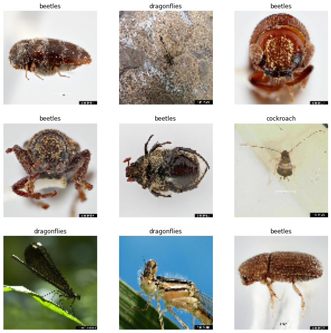
Even the images have been resized, it does not seem to affect the classification.
Data Preprocessing
I first encode the labels of into numeric values. LabelEncoder encode labels with a value between 0 and K_classes-1 where K is the number of distinct labels. To save memory and space, I generated many batches of size 32 from the training set, which will be used in the backpropagation later.
batch_size = 32

## encode labels
le = LabelEncoder()
le.fit(y_train)
y_train = le.transform(y_train)
y_test = le.transform(y_test)

X_train_tensor = torch.Tensor(np.array(X_train) / 255) # transform to torch tensor
y_train_tensor = torch.Tensor(y_train).long()
X_test_tensor = torch.Tensor(np.array(X_test) / 255)
y_test_tensor = torch.Tensor(y_test).long()

train_dataset = torch.utils.data.TensorDataset(X_train_tensor, y_train_tensor) # create datset
test_dataset = torch.utils.data.TensorDataset(X_test_tensor, y_test_tensor)

# create data loader
train_loader = torch.utils.data.DataLoader(dataset=train_dataset, batch_size=batch_size, shuffle=True)
test_loader = torch.utils.data.DataLoader(dataset=test_dataset, batch_size=batch_size, shuffle=True)
Create the CNN model
As input, a CNN takes tensors of shape (image_height, image_width, color_channels), ignoring the batch size. If you are new to these dimensions, color_channels refers to (R,G,B). In this example, I configure our CNN to process inputs of shape (84, 84, 3). The model architecture (see figure below) is made on the principle of convolutional neural networks. It consists of 3 groups of layers, where the convolution layers (Conv 2D) alternate with the nonlinear layers (Relu) and the pooling layers (Max Pooling 2D). It then follows 2 tightly bound layers (Dense).

class CNN(nn.Module):
    def __init__(self, in_channels, out_channels):
        super(CNN, self).__init__()
        self.conv1 = nn.Conv2d(in_channels=in_channels, out_channels=16, kernel_size=3, stride=2, padding=1, bias=True)
        self.conv2 = nn.Conv2d(in_channels=16, out_channels=64, kernel_size=3, stride=1, padding=0, bias=True)
        self.fc1   = nn.Linear(in_features=64 * 9 * 9, out_features=256)
        self.fc2   = nn.Linear(in_features=256, out_features=84)
        self.fc3   = nn.Linear(in_features=84, out_features=out_channels)

    def forward(self, x):
        x = F.relu(self.conv1(x))
        x = F.max_pool2d(x, 2)
        x = F.relu(self.conv2(x))
        x = F.max_pool2d(x, 2)
        x = x.view(x.size(0), -1)
        x = F.relu(self.fc1(x))
        x = F.relu(self.fc2(x))
        x = self.fc3(x)
        return x
Train the model
When the preparation is complete, the code fragment of the training follows:
def train(model, device, train_loader, criterion, optimizer, epoch):
    train_loss = 0
    correct = 0
    model.train()
    for batch_idx, (data, target) in enumerate(train_loader):
        data, target = data.to(device), target.to(device)
        data = Variable(data.reshape(-1, 3, 84, 84))
        #print(data.shape)
        target = Variable(target)
        optimizer.zero_grad()
        output = model(data)
        loss = criterion(output, target)
        loss.backward()
        optimizer.step()
        train_loss += loss.item()  # sum up batch loss
        pred = output.argmax(dim=1, keepdim=True) # get the index of the max log-probability
        correct += pred.eq(target.view_as(pred)).sum().item()
        if batch_idx == len(train_loader)-1:
            print('Epoch {}, Training Loss: {:.4f}'.format(epoch, train_loss/(batch_idx+1)))
    acc = correct / len(train_loader.dataset)
    return(acc)


def test(model, device, test_loader, criterion, epoch):
    model.eval()
    test_loss = 0
    correct = 0
    with torch.no_grad():
        for data, target in test_loader:
            data, target = data.to(device), target.to(device)
            data = Variable(data.reshape(-1, 3, 84, 84))
            target = Variable(target)
            output = model(data)
            test_loss += criterion(output, target).item()
            pred = output.argmax(dim=1, keepdim=True)
            correct += pred.eq(target.view_as(pred)).sum().item()
    acc = correct / len(test_loader.dataset)
    #test_loss = (test_loss*batch_size)/len(test_loader.dataset)
    print('Test{}: Accuracy: {:.4f}%'.format(epoch, 100. * acc))
    return(acc)
device = 'cuda'
device = torch.device(device)
num_epochs = 30
in_channels = 3
out_channels = 3
model = CNN(in_channels, out_channels).to(device)
criterion = nn.CrossEntropyLoss()
#optimizer = optim.SGD(model.parameters(),lr=0.01,momentum=0.9)
optimizer = optim.Adam(model.parameters(),lr=0.001)
train_acc = []
test_acc = []
for epoch in range(1, num_epochs + 1):
train_acc.append(train(model, device, train_loader, criterion, optimizer, epoch))
acc = test(model, device, test_loader, criterion, epoch)
test_acc.append(acc)
if epoch == 1 or old < acc:
torch.save(model.state_dict(), 'ckpt_cnn.pth')
old = accResults
The graph below shows the intersection of training accuracy and test accuracy. Test accuracy sows the ability of the model to generalize to new data. Test dataset contains only the data that the model never sees during the training and therefor cannot just memorize. If your training data accuracy keeps improving while your test data accuracy gets worse, you are likely in an overfitting situation, i.e. your model starts to basically just memorize the data. It can be seen that after 15 epochs the test accuracy is over 80%, it shows the ability of the model to generalize to new data.
plt.figure(figsize=(12,4))
plt.plot(list(range(len(train_acc))), train_acc, color='blue', label='training accuracy')
plt.plot(list(range(len(test_acc))), test_acc, color='darkorange', label='test accuracy')
plt.legend(loc='upper left', bbox_to_anchor=(1.02, 1), borderaxespad=0)
plt.xlabel('iterations')
plt.ylabel('classification accuracy')
plt.grid()
plt.xlim(0, len(train_acc))
plt.xticks(list(range(0, len(train_acc), 2)),list(range(1, len(train_acc)+1, 2)), fontsize=14);
plt.show()
Let's see a sample of data from the test set with the true labels and the predictions.
model = CNN(in_channels, out_channels).to(device)
model.load_state_dict(torch.load('ckpt_cnn.pth'))

## show samples from the test set
f, axarr = plt.subplots(3,3, figsize = (12,12))
data, label = next(iter(test_loader))
data = data[:9].to(device)
data = Variable(data.reshape(-1, 3, 84, 84))
output = model(data)
pred = output.argmax(dim=1, keepdim=True)
data = data.detach()
label = label.detach()
pred = pred.detach()
label = le.inverse_transform(label.cpu().numpy().ravel())
pred = le.inverse_transform(pred.cpu().numpy().ravel())

for i in range(9):
    axarr[i // 3, i % 3].imshow(see_image(data[i].cpu().numpy().reshape(84, 84, 3)))
    axarr[i // 3, i % 3].set_title(f'True:{label[i]} \n Prediction:{pred[i]}')
    axarr[i // 3, i % 3].axis('off')
pass
The model makes mistakes on the second and the sixth images. For the second one, it is easy for humans to determine it is a cockroach. However, for the sixth one, even for humans, it is difficult to distinguish.
Conclusion
In this article, I assembled and trained a CNN model to classify images of three insects. I have tested and the model does work okay (~80%) for a small number of insect images. I measured how the accuracy depends on the number of epochs in order to detect potential overfitting issues. I found that about 15 epochs are enough for a successful training of the model.
My next step will be to try the model on a larger insect dataset and try to apply it to practical tasks. I would also like to try other neural network design to learn how to achieve higher efficiency and accuracy in various problems.
