
Implementation of First-order Optimization Methods (PyTorch)
In this post, I would like to share my implementation of several famous first-order optimization methods. I know that these methods have been implemented very well in many packages, but I hope my implementation can help you understand the ideas behind it.
Suppose we have \(N\) data examples and the parameters \(\mathbf{w} \in \mathcal{R}^D\).
For convenience, I first write a class named optimizer.
class optimizer:
    def __init__(self):
        pass
    def set_param(self, parameters):
        self.parameters = parameters
        return self
    def step(self):
        raise Exception("Not implemented")
1. (Stochastic) Gradient Descent

Note that underlying i.i.d. assumption, \(\mathbb{E}_{p(i_k)} [\nabla f_{i_k} (\mathbf{w}_k)] = \frac{1}{N} \sum^N_{i=1} \nabla f_{i} (\mathbf{w}_k)\) . This means that \(\frac{1}{N} \sum^N_{i=1} \nabla f_{i} (\mathbf{w}_k)\) is an unbiased estimator of \(\mathbb{E}_{p(i_k)} [\nabla f_{i_k} (\mathbf{w}_k)]\).
The performance of Stochastic Gradient Descent (SGD) and Gradient Descent (GD) are shown in the picture below. Even though gradient descent algorithms may take a much longer time, its direction is more accurate.

However, this iterative algorithms are expensive:
- Gradient descent takes:
- \(\mathcal{O}(N)\) to estimate gradients
- \(\mathcal{O}(1)\) to update the parameters
- Stochastic gradient descent takes:
- \(\mathcal{O}(1)\) to estimate gradients
- \(\mathcal{O}(1)\) to update the parameters
- Newton's method (classical optimization approach) takes:
- \(\mathcal{O}(N)\) to estimate gradients and \(\mathcal{O}(ND^2)\) to estimate Hessian
- \(\mathcal{O}(D^3)\) to update the parameters
It is easy to see that for GoogLeNet image classifier on the ImageNet dataset, with \(N=10^6\) and \(D \cong 5\times 10^6\), GD is nearly impossible.
class SGD(optimizer):
    def __init__(self, lr):
        self.lr = lr
    def step(self):
        for param in self.parameters:
            param.data -= self.lr * param.grad.data
The limitations of the stochastic gradient method are:
- constants (and hence step sizes) are usually unknown
- variance in the gradient estimation limits convergence (much of the recent literature discuss ways of minimizing variance)
- does not utilize the curvature in space, can be very poorly conditioned.
2. Momentum method
Classically, momentum "dampens" the highly oscillatory terms.

class SGD_Momentum(optimizer):
    def __init__(self, lr, beta):
        self.lr = lr
        self.beta = beta
        self.m = None
    def step(self):
        if self.m is None:
            self.m = [torch.zeros_like(param) for param in self.parameters]
        for i, param in enumerate(self.parameters):
            mm = self.beta * self.m[i] + param.grad.data
            self.m[i] = mm
            param.data -= self.lr * mm
3. Nesterov’s accelerated gradient (NAG) method
Nesterov methods invented originally by Yurii Nesterov is used for acceleration of the first order methods.
In addition to the gradient information from the previous iteration, gradients from other iteration(s) are contributed with appropriate weights to the calculation of the current estimate of the parameter.
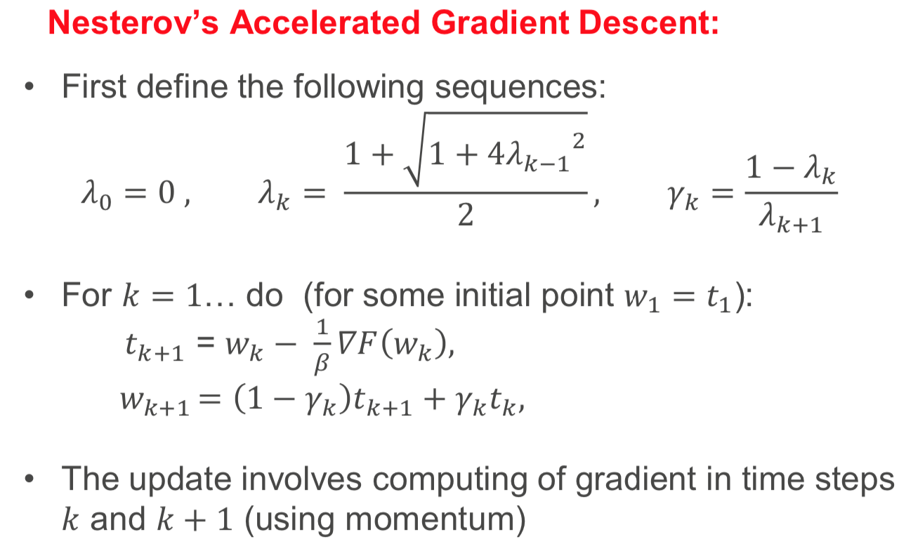
class SGD_NAG(optimizer):
    def __init__(self, lr, beta):
        self.lr = lr
        self.beta = beta
        self.v = self.t = None
    def step(self):
        if self.v is None:
            self.v, self.t = zip(*[(torch.zeros_like(param), param.data) for param in self.parameters])
            self.v, self.t = list(self.v), list(self.t)
        for i, param in enumerate(self.parameters):
            m = 1 - self.v[i]
            self.v[i] = (1 + torch.sqrt(1 + 4 * self.v[i]**2)) / 2
            mm = m / self.v[i]
            t1 = self.t[i]
            self.t[i] = param.data - 1 / self.beta * param.grad.data
            param.data = (1 - mm) * t1 + mm * t1
4. RMSprop Algorithm
Note that RMSprop algorithm does not improve the convergence rate, but it can improve optimizations constants. Since SGD methods are very sensitive to the step size sequences, adaptive methods like RMSprop is robust to the step size sequences, so we can use the same settings across many models and datasets.
The key idea is that sparsely occurring features may be very informative - only decrease step size when information relating to that parameter is seen. This is provably improves regret bounds compared to online (stochastic) gradient descent.

RMSprop algorithm will converge if \(\alpha \rightarrow 0\) with at rate \(t^{1/2}\). The typical step size to use is \(\alpha \cong 10^{-3}\).
class SGD_RMSprop(optimizer):
    def __init__(self, lr, beta, eps, r):
        self.lr = lr
        self.beta = beta
        self.eps = eps
        self.r = r
        self.m = None
    def step(self):
        if self.m is None:
            self.m = [torch.zeros_like(param) for param in self.parameters]
        for i, param in enumerate(self.parameters):
            self.m[i] = self.beta * self.m[i] + (1-self.beta) * torch.square(param.grad.data)
            eta = self.r / (torch.sqrt(self.m[i]) + self.eps)
            param.data -= self.lr * eta * param.grad.data
The limitations of RMSprop:
- there is no convergence guarantee
- no inclusion of momentum
In practive, RMSprop has been largely replaced by the ADAM optimizer, which can address these issues.
5. ADAM Algorithm
ADAM was inspired by RMSprop, if \(\beta_1=0\), then they are very similar algorithms. And ADAM has a provale regret bound under a decreasing step size. The typical parameters for ADAM are \( \alpha = 10^{-3}, ~\beta_1 = 0.9, ~\beta_2 = 0.999. Note that \)\beta_1\( going higher will reduce the variance of gradients, but can add bias. \)

class SGD_Adam(optimizer):
    def __init__(self, lr, betas, eps):
        self.lr = lr
        self.beta1 = betas[0]
        self.beta2 = betas[1]
        self.eps = eps
        self.m = self.v = None
        self.t = None
    def step(self):
        if self.t is None:
            self.t = 0
        if self.m is None:
            self.v, self.m = zip(*[(torch.zeros_like(param), torch.zeros_like(param)) for param in self.parameters])
            self.v, self.m = list(self.v), list(self.m)
        for i, param in enumerate(self.parameters):
            self.t = self.t + 1
            self.m[i] = self.beta1 * self.m[i] + (1-self.beta1) * param.grad.data
            self.v[i] = self.beta2 * self.v[i] + (1 - self.beta2) * torch.square(param.grad.data)
            mc = self.m[i] / (1 - np.power(self.beta1, self.t))
            vc = self.v[i] / (1 - np.power(self.beta2, self.t))
            param.data -= self.lr * mc / (torch.sqrt(vc) + self.eps)
6. Comparison


- Stochastic gradient descent methods are effective at quickly obtaining a reasonable solution.
- Stochastic gradient descent will converge to the optimum if given enough time.
- will converge to a fixed point in nonconvex problems as well.
- Adding in adaptive higher order information can reduce parameter tuning and account for curvature information.
- Many tuning parameters within these algorithms
- hopefully their meaning and how to set them is clearer now.
Thanks for reading.
